The Bootstrap Theorem: Creating Empirical Distributions
Blake Taylor
April 12, 2005
Introduction
When regression coefficients or other statistics are calculated from a data sample, the distribution of the estimates is often based on asymptotic approximations or other theoretical assumptions. The values of the standard errors and confidence intervals, which are derived from these approximate distributions, are then used to determine the accuracy of the estimates and the interval over which confidence can be placed; however, if the standard errors or confidence intervals are inaccurate, too much or too little confidence will be placed on the estimates. This can especially occur when basic assumptionsŚsuch as the distribution of the estimatesŚdonÆt hold.
The bootstrap method was developed in order to help solve this problem by obtaining an understanding of the distribution of a sample. In the bootstrap, the sample data is treated as the population. ōPseudo dataö is then randomly generated from the sample data to obtain a distribution. This distribution can then be used to obtain standard errors, confidence intervals, and other statistics; under certain conditions the bootstrap can provide standard errors and other statistics that are more accurate than a theoretical approximation would yield (Hall 1996).
This paper will discuss the bootstrap method, why it is used, and will give two examples of its useŚa sample taken from the standard normal distribution and a linear regression model dealing with violent crime across states.
Description of the Bootstrap
The bootstrap method is applied by taking B random samples with replacement from the sample data set. Each of these random samples will be the same size n as the original set, but because the elements are randomly selected with replacement, some of the original values will be selected more than once while others will be left out. This causes each resample to randomly depart from the original sample (Cugnet 1997). When the statistic of interest Gb is calculated for each resample, it will vary slightly from the original sample statistic, enabling us to construct a relative frequency histogram of the statistic of interest in order to gain an understanding of its distribution.
Thus, the bootstrap method consists of five basic steps:
1. Obtain a sample of data size n from a population.
2. Take a random sample of size n with replacement from the sample set.
3. Calculate the statistic of interest Gb for the random sample.
4. Repeat steps 2 and 3 a large number B times (usually over 1000).
5. Create a relative frequency histogram of the B statistics of interest Gb by placing a probability of 1/B at each estimated statistic.
If the sample is a good indicator of the population, the bootstrap estimate of the population statistic will be similar to the original sample. As B approaches infinity the bootstrap estimate of the statistic of interest will approach the population statistic.
ApplicationŚSample of Standard Normal Distribution
We will first look at an application of the bootstrap on a sample data set from the standard normal distribution. The data set consists of a random sample of n=300 values which was obtained the SAS function rannor(), which generates random numbers from the standard normal distribution.
B = 2000 samples with replacement of size n=300 were drawn from the original 300 data samples. The mean and standard deviation were then computed for each bi. The following histograms of the mean and the SD resulted by placing a probability of 1/B for each bi statistic:
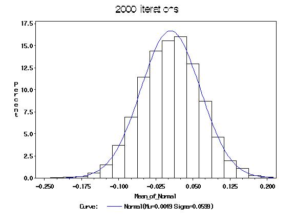
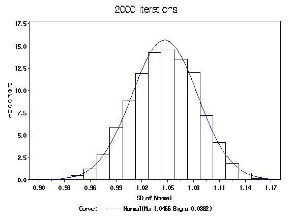
This table shows the true mean and standard deviation of the population (the standard normal distribution) and the bootstrap-estimated mean and standard deviation of the sample.
| Standard Normal |
|---|
| | Mean | SD of estimate | SD | SD of estimate |
|---|
| Theoretical Values | 0 | | 1 | |
| Bootstrap (B=2000) | 0.00486 | 0.05987 | 1.04656 | 0.03825 |
The Bootstrap comes close to predicting the true values of the population due to the fact that the sample is a good approximation of the population. The estimates are similar to the sampleÆs estimates.
Application of the Bootstrap to Linear Regression
A method called the pairs bootstrap can be applied to the linear regression model Y = X ▀ + e. The bootstrap samples are obtained by sampling with replacement n observations (rows) from the data vector Y and matrix X. Each sample bi of n rows from the matrices is then regressed to produce B estimates of each parameter ▀i. A histogram is constructed by placing a probability of 1/B at each parameter.
Confidence intervals for the bootstrap estimates can be obtained by sorting the data by ascending order of ▀i* and then selecting the (a * B)th and ((1- a) * B)th observations for the lower and upper bounds. Because the histograms are not symmetrically distributed, these are not always the minimum length confidence intervals. In order to obtain CIÆs of minimum length, find the minimum value of ▀i* for
b1+((1-2a)*B) ¢ b1, b2+((1-2a)*B) ¢ b2, ģ , bB ¢ bB-((1-2a)*B)
To construct an example of the paired bootstrap, data was taken for 50 states from the following model:
VC = ▀0 + ▀1(MA) + ▀2(Pov) + ▀3(S) + e
Where VC is violent crimes per 100,000 population, MA is the percentage of the population living in a metropolitan area, Pov is the percentage of the population living under the poverty level, and S is the percentage of families headed by a single parent.
| Descriptive Statistics |
|---|
| VC | MA | Pov | S |
|---|
| Mean | 566.7 | 66.7 | 14.0 | 11.1 |
| Max | 1206 | 100 | 26.4 | 14.9 |
| Min | 82 | 24 | 8.0 | 8.4 |
The paired bootstrap was created using B = 2000 resamples of n = 50 observations. A 95% minimum length confidence interval was obtained by sorting the data by ▀i* and then selecting the ▀i* where bi and bi+1950 had the least difference. A comparison of the bootstrap with the simple regression follows.
| Regular OLS Regression | Bootstrap (B=2000) |
|---|
| Parameter | 95% Confidence Interval | Parameter | 95% Confidence Interval |
|---|
| Variable | Estimate | Lower Bd. | Upper Bd. | Estimate | Lower Bd. | Upper Bd. |
|---|
| Intercept | -1197.54 | -1560.84 | -834.24 | -1215.09 | -1622.77 | -831.37 |
| ma | 7.71 | 5.48 | 9.95 | 7.65 | 5.14 | 10.23 |
| pov | 18.28 | 5.93 | 30.63 | 20.13 | 7.31 | 36.15 |
| s | 89.4 | 53.50 | 125.3 | 89.08 | 40.55 | 128.78 |
All of the regular OLS estimates were significant at the 95% level.
The distribution of the bootstrap parameter estimates were compared with a Normal Distribution with using the Chi-square goodness of fit test:
Chi^2 = SUM:(Oi ¢ Ei)2/Ei
where Oi is the observed frequency for bin i (of the histogram) and Ei is the expected frequency for bin i. The expected frequency Ei = N(F(Yu) ¢ F(Yl)) where F is the cumulative distribution function for the Normal curve (NIST 2005). If ?2 > ?2(a, k-c) then the null hypothesis, that the bootstrap parameter estimate is normally distributed, is rejected. The following ?2 values were obtained for the parameters:
| Chi-square Goodness of Fit |
|---|
| Parmeter | Chi^2 | d.f. | P Value |
|---|
| Intercept | 70.18 | 16 | <0.0001 |
| ma | 10.26 | 15 | 0.8013 |
| pov | 692.61 | 15 | <0.0001 |
| s | 2154.75 | 15 | <0.0001 |
The estimate of the bootstrap parameter of ma, ▀1, was the only significant fit according to the Chi-square test. The following shows the bootstrap histogram against the regular OLS regression parameter ▀1~N[▀1 = 7.71, Var = 1.21]:
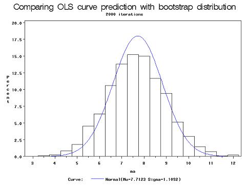
The rejection of the Chi-square goodness of fit test of the other three parameters (▀0, ▀2, ▀3) was most likely due to the small sample size and outliers among the data. The effect of outliers among a small data set can be further demonstrated by adding another observation, the data for the District of Columbia, to the original data set of the 50 states, resulting in n=51. The District of Columbia contains VC=2922, MA=100, Pov=26.4, and S=22.1Śall of these are maximum values over the 51 observations.
Now the same analysis will be conducted with the District of Columbia observation included (i.e.: 2000 bootstrap iterations of the regression model, only with n=51 instead of 50):
| Regular OLS Regression | Bootstrap (B=2000) |
|---|
| Parameter | 95% Confidence Interval | Parameter | 95% Confidence Interval |
|---|
| Variable | Estimate | Lower Bd. | Upper Bd. | Estimate | Lower Bd. | Upper Bd. |
|---|
| Intercept | -1666.44 | -1963.88 | -1369.00 | -1551.28 | -2001.03 | -991.57 |
| ma | 7.83 | 5.30 | 10.35 | 7.68 | 4.93 | 10.67 |
| pov | 17.68 | 3.72 | 31.64 | 18.60 | 5.07 | 35.59 |
| s | 132.41 | 101.22 | 163.60 | 121.93 | 59.17 | 166.80 |
All of the regular OLS estimates were significant at the 98% level. Notice the large discrepancy between the confidence intervals of the parameters of the Intercept and S. The following chart shows the OLS prediction of the intercept, ▀0~N[▀0 = -1666.44, Var = 21859.62] against the histogram of the bootstrap estimate of ▀0:
The bootstrap estimate of ▀0 takes on a seemingly bimodal distribution (as does ▀0*). This demonstrates a limit of the bootstrap: it must be used with a large enough sample size to reflect the true population. In this case, each bootstrap iteration that included one or more of the District of Columbia observations was shifted to the left, while those without DC observations remained near the 50 state mean. Although there werenÆt any observations with outliers to the same extreme in the original 50 state data set, the sample size wasnÆt great enough to compensate for any that were near the minimum or maximum values.
In addition to obtaining the empirical distribution of the parameters, the bootstrap method can also be used to obtain the distribution of the t-statistics, which should be normally distributed. The same method is used, only that t-stats are computed for each bi and then used to construct the histogram.
Using the 50 state (not including DC) data, the following chi-square goodness of fit results were found:
| Chi-square Goodness of Fit |
|---|
| T-stat | Chi^2 | d.f. | P Value |
|---|
| Intercept | 6.75 | 17 | 0.9866 |
| ma | 1.45 | 14 | >0.9999 |
| pov | 3.63 | 17 | 0.9997 |
| s | 2.81 | 19 | >0.9999 |
We cannot reject the null hypothesis that any of the t-stat distributions were not normally distributed.
For a final example, the paired bootstrap will be used to determine confidence intervals of heteroskedastic data. The data was generated in the following manner:
- X = [1, 2, 3, ģ, 500]Æ
- Y = X + e ~ N(0, 1), e being generated by a standard normal distribution random number generator.
- yi = yi + (yi * 0.5 * r), r being a random number in the standard normal distribution. This gives the error term a larger variance as the value of yi increases.
A modified White test was performed by regressing the squares of the residual estimates ui* on the predicted values of y and y2. The F-statistic was 48.73, so we conclude that there is sufficient evidence to reject the null hypothesis, that ▀0 = ▀1 = 0 at the 99% level, and therefore heteroskedasticity is present:
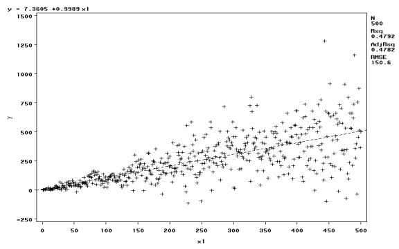
For Y = X▀ + e, the ordinary least squares regression should yield inefficient but consistent and unbiased estimates of ▀; thus ▀0 ś 0 and ▀1 ś 1. The following resulted from the OLS regression and a bootstrap with B = 2000 and n = 500:
| Regular OLS Regression | Bootstrap (B=2000) |
|---|
| Parameter | Standard | 95% Confidence Interval | Parameter | Standard | 95% Confidence Interval |
|---|
| Variable | Estimate | Error | Lower Bd. | Upper Bd. | Estimate | Error | Lower Bd. | Upper Bd. |
|---|
| Intercept | 7.3605 | 13.4899 | 19.1435 | 33.8646 | 7.04226 | 8.92782 | 9.7102 | 24.537 |
| X1 | 0.9989 | 0.0467 | 0.9072 | 1.0906 | 1.00075 | 0.052948 | 0.89602 | 1.09682 |
| Chi-square Goodness of Fit |
|---|
| Parameter | Chi^2 | d.f. | P Value |
|---|
| Intercept | 19.8712 | 15 | 0.1769 |
| X1 | 7.64846 | 16 | 0.9586 |
Both of the bootstrap estimates of the parameter distributions were normally distributed. The confidence interval for the bootstrap estimate of ▀0 was actually tighter, or more efficient, than that of the regular OLS regression:
Conclusion
The bootstrap method is very useful in obtaining empirical distributions to compare with theoretical distributions. In certain cases of a small sample, such as the violent crime example, it is not dependable but can give a picture of how outliers are affecting the estimates. For heteroskedastic data, bootstrap estimates can sometimes be more efficient than ordinary least squares regression.
References
- Andrews, Donald W. K. and Moshe Buchinsky. A Three-Step Method for Choosing the Number of Bootstrap Repetitions. Econometrica, Vol. 68, No. 1 (Jan, 2000), 23-51.
- Brownstone, David and Robert Valleta. The Bootstrap and Multiple Imputations: Harnessing Increased Computing Power for Improved Statistical Tests. The Journal of Economic Perspectives, Vol. 15, No. 4 (Autumn, 2001), 129-141.
- Cugnet, Pierre. Confidence Interval Estimation for Distribution Systems Power Consumption by using the Bootstrap Method. Digital Library and Archives. 15 July 1997. Virginia Tech. 20 February 2005 http://scholar.lib.vt.edu/theses/available/etd-61697-14555/.
- Eakin, B. Kelly, Daniel P. McMillen, and Mark J. Buono. Constructing Confidence Intervals Using the Bootstrap: An Application to a Multi-Product Cost Function. The Review of Economics and Statistics, Vol. 72, No. 2 (May, 1990), 339-344.
- Hall, Peter and Joel L. Horowitz. Bootstrap Critical Values for Tests Based on Generalized-Method-of-Moments Estimators. Econometrica, Vol. 64, No. 4 (July, 1996), 891-916.
- NIST/SEMATECH e-Handbook of Statistical Methods, http://www.itl.nist.gov/div898/handbook/, 11 April 2005.
|
|