An Empirical Evaluation of the Capital Asset Pricing Model
Blake Taylor
December 8, 2005
Introduction
The Capital Asset Pricing Model, which was developed in the mid 1960's, uses various assumptions about markets and investor behavior to give a set of equilibrium conditions that allow us to predict the return of an asset for its level of systematic (or nondiversifiable) risk. The CAPM uses a measure of systematic risk that can be compared with other assets in the market. Using this measure of risk can theoretically allow investors to improve their portfolios and managers to find their required rate of return. In this paper, an empirical test is conducted using data from the S&P 500 to determine if the CAPM is valid.
Review of Literature
Harry Markowitz's paper, "Portfolio Selection", established “the idea of diversifying a portfolio of stocks in order to produce the maximum potential returns given the amount of risk an investor is prepared to take on" [1]. Twelve years later William Sharpe, John Lintner, and Jan Mossin developed the CAPM in a series of articles [2].
After the CAPM was developed, many empirical tests of the model were conducted using proxies for the different variables. Several of these showed that the CAPM didn't hold in many situations and was often inaccurate or unsuitable in predicting asset values. In 1977 Richard Roll asserted that the CAPM holds theoretically but is hard to test empirically since stock indexes and other measures of the market are poor proxies for the CAPM variables. This came to be known as Roll's critique.
The biggest assault on the CAPM came from French and Fama [3]. Using a large sample of cross-sectional stock data including many small-cap stocks and stocks with large book values, they analyzed the accuracy of the CAPM and looked for other factors that explained stock prices (besides systematic risk). They found that while the CAPM's measure of systematic risk was unreliable, firm size and book to market value ratios were more dependable. Even so, French and Fama's findings have encountered a great deal of criticism. For example, using better econometric techniques might lead to better results for the CAPM. Just as Roll stated, the CAPM also has many values for which proxies must be found, and the proxies are often inadequate. It is easiest to test the CAPM ex post, although it would be better if an ex ante trial could be realized. Similarly, data mining can lead to conclusions that have no theoretical base.
Today the CAPM is still widely taught because of the insights it gives into capital markets and because it is sufficient for many important applications.
Theory
Various assumptions must be defined in order to arrive at the CAPM equilibrium, these include:
- Investors maximize expected utility of wealth.
- Investors have homogenous expectations and use the same input list.
- Markets are frictionless—the borrowing rate is equal to the lending rate.
- There are many investors, each with an endowment of wealth which is small compared to the total endowment of all investors (investors are price-takers).
- All investors plan for one identical holding period.
- There are no taxes or transaction costs [4].
Given these assumptions we can build the CAPM model and arrive at the prevailing equilibrium, which is summarized in the following paragraphs.
First, all investors will choose the market portfolio, M, as their optimal portfolio. M includes all assets in the economy, with each asset weighted in the portfolio in proportion to its weight in the economy. Since all investors have the same expectations and use the same input list, they will each choose an identical risky portfolio, which is the portfolio on the efficient frontier that lies on the tangency line drawn from the risk free asset. If any asset were left out of that portfolio its demand would be zero and therefore its price would approach zero. Seeing this, all investors would adjust their portfolio to include this asset until it had a price that would reflect its amount of risk. Thus we can see that all assets will be included in M.
Second, the market portfolio, M, lies on the efficient frontier and is the tangent asset to the risk-free asset. Since investors all have identical input lists and all hold M, all information about assets in the market is incorporated into M, resulting in an efficient portfolio. Each individual investor will then choose to allocate his wealth between M and the risk free asset, or in other words the Capital Allocation Line runs between the risk free asset and the portfolio M.
Third, the risk premium on the market portfolio will be proportional to its own risk and the degree of risk aversion of the average investor [5]. Each investor chooses a proportion b to invest in the market portfolio M and a proportion 1-b to invest in the risk free asset such that
b = [E(rMarket) – rfree] / [AsMarket^2]
where E(rMarket) is the expected return to the market portfolio, rf is the risk free return, A is a measure of risk aversion, and sMarket^2 is the market portfolio's risk. Since any borrowing is offset by lending, b for the average investor is equal to 1. From this we can show that
E(rMarket) – rfree = AsMarket^2
Fourth, the risk premium on individual assets [E(ri) – rf] will be proportional to the risk premium on the market portfolio and the beta coefficient of the asset relative to the market portfolio where beta is defined as
ß = [Cov(ri, rMarket)] / sMarket^2
The correct risk premium of an asset must be determined by the contribution of the asset to the risk of the portfolio. As the number of assets in the market portfolio gets very large, a given asset's contribution to the risk of the portfolio depends almost entirely on its covariance with other assets in the portfolio and its weight in the portfolio, while the contribution of its own risk (or the asset's variance) to the risk of the portfolio approaches zero. Thus, as the number of assets in the portfolio gets very large,
Cov(ri, rMarket) = Cov(ri, SUM:wkrk)
Consequently for specific assets in the market portfolio the correct measure of risk is their covariance with the market portfolio. An asset's reward-to-risk ratio would be
wi[E(ri) – ri] / wiCov(ri, rmarket) = [E(ri) – ri] / Cov(ri, rmarket)
Because we are in equilibrium, all assets must offer equivalent reward-to-risk ratios, otherwise investors would choose assets with superior ratios to invest in. This means that the reward-to-risk ratio of all assets must be equal to the reward-to-risk ratio of the market portfolio, that is,
[E(ri) – rfree] / Cov(ri, rMarket) = [E(rMarket) – rfree] / sMarket^2
or E(ri) = rfree + ßi[E(rMarket) – rfree]
This equation is the most common form of the CAPM. ßi is an appropriate measure of risk for an asset since it measures the asset's contribution to the risk of the market portfolio. ßi is proportional to the premium of the asset—an asset's premium depends on its contribution to the risk of the market portfolio.
Graphically, we can represent the return-beta relationship through the security market line, or the SML. At ß = 0 the line will intersect the y-axis at the risk free rate. At ß = 1 the line will be at E(rM) on the y-axis since Cov(rM, rM) / s2M = 1. Also, it can be shown that the slope of the SML is equal to the expected excess returns to the market (E(rM) – rf).
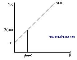
In equilibrium, all assets will lie on the SML because they will have an appropriate return-beta relationship. However, if we depart from equilibrium some assets will not be correctly priced. If an asset is overpriced it will lie below the SML since it will provide an expected return less than what is determined by the SML given its risk (beta). If an asset is underpriced it will lie above the SML since its return will be greater than what the SML determines.
The CAPM gives investors a tool for determining their investment decisions. By estimating a SML and plotting an asset, the investor can determine whether the asset is over or underpriced and make investment decisions based on that knowledge.
Description of Data
In order to test the CAPM model, data has been collected for monthly intervals between January 1995 and December 2004 [6]. The equation
E(ri) = rf + ßi[E(rMarket) – rf]
will be tested by observing the 120 monthly holding period rate of returns on 20 stocks within the S&P 500 index. The S&P 500 will be used as an approximation of the market and monthly rates of the 3-month Treasury Bill in the Secondary Market will be used as an approximation for the risk-free rate.
Methods and Results
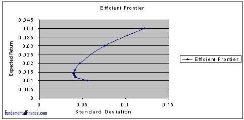
Before testing the above equation, a 120 x 20 matrix consisting of the stock returns was created, followed by a 20 x 20 variance-covariance matrix of the stock returns. Another 20 x 20 matrix was then created and which weighted the variance covariance matrix by the stock weights in a given portfolio. From this matrix a portfolio variance and standard deviation could be derived. Finally, the portfolio weights were adjusted until the standard deviation was minimized and the expected portfolio return was found. This gave the minimum risk (standard deviation) portfolio, with an expected return and standard deviation of (0.0142, 0.0397).
After plotting this point, a new portfolio was found which minimized standard deviation for a given expected return. This process was repeated for various values and each point was plotted, resulting in the following efficient frontier:
After finding this frontier, a 120 x 21 matrix was constructed consisting of the 20 columns of excess stock returns (rit – rft) and 1 column of excess market returns (rMt – rft) in order to test the expected return-beta relationship predicted by the CAPM. Each excess stock return was then regressed on the excess market returns to estimate the beta coefficient as follows:
rit – rft = ai + bi(rMarket t – rft) + eit
To estimate expected excess returns, the sample average excess returns were taken for each stock as well as the market. The values of bi are estimates of the true beta coefficients for the 20 stocks during the sample period. The residual ei of each estimate was squared in order to estimate the nonsystematic risk for each stock [7].
Now the SML will be constructed and its coefficients estimated to verify that our CAPM is valid. The coefficient of beta is estimated by regressing estimated expected excess stock returns on the estimates of beta. The estimated nonsystematic risk for each stock will also be included in the regression to see whether it is correlated with the excess returns.
S(rit – rft)/n = a0 + a1bi + a2*ei^2 + ui
If the CAPM is valid, then three conditions are satisfied:
- a0 = 0, there is no risk premium for bearing nonsystematic risk,
- a1 = S(rmarket – rf)/n, beta times the excess market return yields the excess stock return,
- a2 = 0, expected excess return is independent of nonsystematic risk.
Testing these hypotheses produced the subsequent results:
| Coef. | Std. Err. | ratio | Result |
| a0 | 0.004409 | 1.77 | Fail to reject at 95% level |
| a1 | 0.004558 | 1.545 | Fail to reject at 95% level |
| a2 | 0.2741 | 0.275 | Fail to reject at 95% level |
Conclusion
The empirical test of the CAPM showed that the CAPM was fairly successful in predicting the price of individual assets. None of the three necessary conditions for a valid model were rejected at the 95% level. Although the CAPM was not perfectly accurate, it still provides a legitimate explanation of asset prices—that they're expected return is proportional to their systematic risk and the expected excess return to the market. The inaccuracies in this and other empirical tests can be improved with better proxies for the market and the risk free rate and better econometric techniques.
Footnotes
- [1] Christopher Farrell, Business Week 2004.
- [2] Zvi Bodie, et al., Investments 282.
- [3] French and Fama, Journal of Finance 1992.
- [4] Zvi Bodie, et al., Investments 282.
- [5] Ibid, 283.
- [6] http://wrds.wharton.upenn.edu and www.research.stlouisfed.org/fred2
- [7] Zvi Bodie, et al., Investments 417.
|
|